Read 101 Excel 2013 Tips, Tricks and Timesavers Online
Authors: John Walkenbach
101 Excel 2013 Tips, Tricks and Timesavers (10 page)


Figure 18-2:
Using an additional column for the bullet characters, or for numbers.
Using SmartArt
Another way to create a bulleted list in Excel is to use SmartArt. Choose Insert⇒Illustrations
➜
SmartArt, and choose the diagram style from the dialog box.
Figure 18-3 shows a “Vertical Bullet List” SmartArt diagram. This object is free-floating and can easily be moved and resized. The example shown here uses minimal formatting, but you have lots of control over the appearance of SmartArt.

Figure 18-3:
Using SmartArt to hold a bulleted list.
Tip 19: Shading Alternate Rows Using Conditional Formatting
When you create a table (using Insert⇒Tables⇒Table), you have the option of formatting the table in such a way that alternate rows are shaded. Alternate row shading can make your spreadsheets easier to read.
This tip describes how to use conditional formatting to obtain alternate row shading for any range of data. It’s a dynamic technique: If you add or delete rows within the conditional formatting area, the shading is updated automatically.
Displaying alternate row shading
Figure 19-1 shows an example. Here’s how to apply shading to alternate rows:
1.
Select the range to format.
2.
Choose Home⇒Conditional Formatting⇒New Rule.
The New Formatting Rule dialog box appears.
3.
For the rule type, choose Use a Formula to Determine Which Cells to Format.
4.
Enter the following formula in the box labeled Format Values Where This Formulas Is True:
=MOD(ROW(),2)=0
5.
Click the Format button.
The Format Cells dialog box appears.
6.
In the Format Cells dialog box, click the Fill tab and select a background fill color.
7.
Click OK to close the Format Cells dialog box, and click OK again to close the New Formatting Rule dialog box.
This conditional formatting formula uses the ROW function (which returns the row number) and the MOD function (which returns the remainder of its first argument divided by its second argument). For cells in even-numbered rows, the MOD function returns
0
, and cells in that row are formatted.
For alternate shading of columns, use the COLUMN function instead of the ROW function.

Figure 19-1:
Using conditional formatting to apply formatting to alternate rows.
Creating checkerboard shading
The following formula is a variation on the example in the preceding section. It applies formatting to alternate rows and columns, creating a checkerboard effect. Figure 19-2 shows the result.
=MOD(ROW(),2)=MOD(COLUMN(),2)

Figure 19-2:
Conditional formatting produces this checkerboard effect.
Shading groups of rows
Here’s another row shading variation. The following formula shades alternate groups of rows. It produces four rows of shaded rows, followed by four rows of unshaded rows, followed by four more shaded rows, and so on. Figure 19-3 shows an example.
=MOD(INT((ROW()-1)/4)+1,2)
For different sized groups, change the 4 to some other value. For example, use this formula to shade alternate groups of two rows:
=MOD(INT((ROW()-1)/2)+1,2)
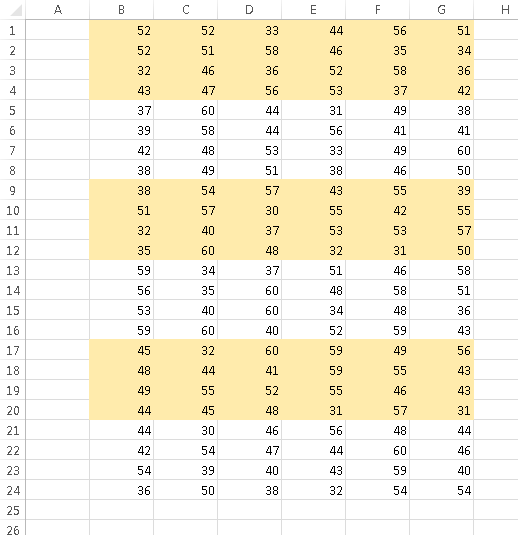
Figure 19-3:
Conditional formatting produces these groups of alternate shaded rows.
Tip 20: Formatting Individual Characters in a Cell
Excel cell formatting isn’t an all-or-none proposition. In some cases, you might find it helpful to be able to format individual characters within a cell.
 This technique is limited to cells that contain text. It doesn’t work if the cell contains a value or a formula.
To apply formatting to characters within a text string, select those characters first. You can select them by clicking and dragging your mouse on the Formula bar, or you can double-click the cell and then click and drag the mouse to select specific characters directly in the cell. A more efficient way to select individual characters is to press F2 first and then use the arrow keys to move between characters and use the Shift+arrow keys to select characters.
When the characters are selected, use formatting controls to change the formatting. For example, you can make the selected text bold, italic, or a different color; you can even apply a different font. If you right-click, the Mini Toolbar appears, and you can use those controls to change the formatting of the selected characters.
Figure 20-1 shows a few examples of cells that contain individual character formatting.
Unfortunately, two useful formatting attributes are not available on the Ribbon or on the Mini Toolbar: superscript and subscript formatting. If you want to apply superscripts or subscripts, open the Font tab in the Format Cells dialog box. Just press Ctrl+1 after you select the text to format.

Figure 20-1:
Examples of individual character formatting.
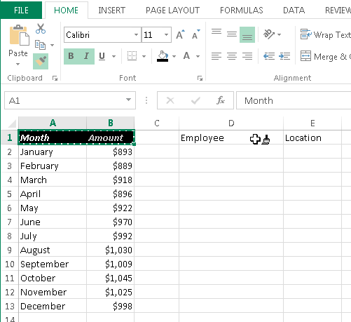
Tip 21: Using the Format Painter
You’ve probably seen that little Format Painter paint brush icon in the Home⇒Clipboard group. It’s an easy way to copy cell formatting — and it’s actually more versatile than you might think.
When you use the Format Painter,
every
aspect of the source range’s formatting is copied, including number formats, borders, cell merging, and conditional formatting.
Painting basics
Here’s how to use the Format Painter tool in its basic form:
1.
Select a cell that contains the formatting that you want to duplicate.
2.
Choose Home⇒Clipboard⇒Format Painter.
The mouse cursor displays a paintbrush to remind you that you’re in Format Painter mode (see Figure 21-1).
3.
Drag the mouse over another range.
4.
Release the mouse button, and the formatting is copied.
In Step 2, you can right-click the selected cell and choose the Format Painter icon from the Mini Toolbar.
Note that the Format Painter is mouse-centric. You cannot use the keyboard to do your painting.