Statistics Essentials For Dummies (9 page)

Interpreting a boxplot
A boxplot can show information about the distribution, variability, and center of a data set.
Distribution of data in a boxplot
A boxplot can show whether a data set is symmetric (roughly the same on each side when cut down the middle), or skewed (lopsided). Symmetric data shows a symmetric boxplot; skewed data show a lopsided boxplot, where the median cuts the box into two unequal pieces. If the longer part of the box is to the right (or above) the median, the data is said to be
skewed right
. If the longer part is to the left (or below) the median, the data is
skewed left
. However, no data set falls perfectly into one category or the other.
In Figure 3-5, the upper part of the box is wider than the lower part. This means that the data between the median (77) and Q
3
(89) are a little more spread out, or variable, than the data between the median (77) and Q
1
(68). You can also see this by subtracting 89 - 77 = 12 and comparing to 77 - 68 = 9. This indicates the data in the middle 50% of the data set are a bit skewed right. However, the line between the min (43) and Q
1
(68) is longer than the line between Q
3
(89) and the max (99). This indicates a "tail" in the data trailing to the left; the low exam scores are spread out quite a bit more than the high ones. This greater difference causes the overall shape of the data to be skewed left. (Since there are no strong outliers on the low end, we can safely say that the long tail is not due to an outlier.). A histogram of the exam data, shown in the graph in Figure 3-6, confirms the data are generally skewed left.
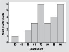
Figure 3-6:
Histogram of 25 exam scores.
A boxplot can tell you whether a data set is symmetric, but it can't tell you the shape of the symmetry. For example, a data set like 1, 1, 2, 2, 3, 3, 4, 4 is symmetric and each number appears the same number of times, whereas 1, 2, 2, 2, 3, 4, 5, 5, 5, 6 is also symmetric but doesn't have an equal number of values in each group. Boxplots of both would look similar in shape. A histogram shows the particular shape that the symmetry has.
Variability in a data set from a boxplot
Variability in a data set that is described by the five-number summary is measured by the
interquartile range
(IQR — see Chapter 2 for full details on the IQR). The interquartile range is equal to Q
3
- Q
1
. A large distance from the 25th percentile to the 75th indicates the data are more variable. Notice that the IQR ignores data below the 25th percentile or above the 75th, which may contain outliers that could inflate the measure of variability of the entire data set. In the exam score data, the IQR is 89 - 68 = 21, compared to the range of the entire data set (max - min = 56). This indicates a fairly large spread within the innermost 50% of the exam scores.
Center of the data from a boxplot
The median is part of the five-number summary, and is shown by the line that cuts through the box in the boxplot. This makes it very easy to identify. The mean, however, is not part of the boxplot, and couldn't be determined accurately from a boxplot. In the exam score data, the median is 77. Separate calculations show the mean to be 76.96. These are extremely close, and my reasoning is because the skewness to the right within the middle 50% of the data offsets the skewness to the left of the outer part of the data. To get the big picture of any data set you need to find more than one measure of center and spread, and show more than one graph, as the ideal report.
variability
(a wider range of values) in that part of the box, not more data. You can't even tell how many data values are included in a boxplot — it is totally built around percentages.
Chapter 4
:
The Binomial Distribution
In This Chapter
Identifying a binomial random variable
A
random variable
is a characteristic, measurement, or count that changes randomly according to some set of probabilities; its notation is X, Y, Z, and so on. A list of all possible values of a random variable, along with their probabilities is called a
probability distribution
. One of the most well-known probability distributions is the binomial.
Binomial
means "two names" and is associated with situations involving two outcomes: success or failure (hitting a red light or not; developing a side effect or not). This chapter focuses on the binomial distribution —when you can use it, finding probabilities for it, and finding the expected value and variance.
Characteristics of a Binomial
A random variable has a binomial distribution if all of following conditions are met:
1. There are a fixed number of trials (
n
).
2. Each trial has two possible outcomes: success or failure.
3. The probability of success (call it
p
) is the same for each trial.
4. The trials are independent, meaning the outcome of one trial doesn't influence that of any other.
Let
X
equal the total number of successes in
n
trials; if all of the above conditions are met,
X
has a binomial distribution with probability of success equal to
p
.
Checking the binomial conditions step by step
You flip a fair coin 10 times and count the number of heads. Does this represent a binomial random variable? You can check by reviewing your responses to the questions and statements in the list that follows:
1. Are there a fixed number of trials?
You're flipping the coin 10 times, which is a fixed number. Condition 1 is met, and
n
= 10.
2. Does each trial have only two possible outcomes — success or failure?
The outcome of each flip is either heads or tails, and you're interested in counting the number of heads, so flipping a head represents success and flipping a tail is a failure. Condition 2 is met.
3. Is the probability of success the same for each trial?
Because the coin is fair the probability of success (getting a head) is
p
= 1//2 for each trial. You also know that 1 - 1//2 = 1//2 is the probability of failure (getting a tail) on each trial. Condition 3 is met.
4. Are the trials independent?
We assume the coin is being flipped the same way each time, which means the outcome of one flip doesn't affect the outcome of subsequent flips. Condition 4 is met.
Non-binomial examples
Because the coin-flipping example meets the four conditions, the random variable
X
, which counts the number of successes (heads) that occur in 10 trials, has a binomial distribution with
n
= 10 and
p
= 1//2. But not every situation that appears binomial actually is binomial. Consider the following examples.
No fixed number of trials
Suppose now you are to flip a fair coin until you get four heads, and you count how many flips it takes to get there. (That is,
X
is the number of flips needed.) This certainly sounds like a binomial situation: Condition 2 is met since you have success (heads) and failure (tails) on each flip; Condition 3 is met with the probability of success (heads) being the same (0.5) on each flip; and the flips are independent, so Condition 4 is met.
However, notice that
X
isn't counting the number of heads, it counts the number of trials needed to get 4 heads. The number of successes (
X
) is fixed rather than the number of trials (
n
). Condition 1 is not met, so
X
does not have a binomial distribution in this case.
More than success or failure
Some situations involve more than two possible outcomes yet they can appear to be binomial. For example, suppose you roll a fair die 10 times and record the outcome each time. You have a series of
n
= 10 trials, they are independent, and the probability of each outcome is the same for each roll. However, you're recording the outcome on a six-sided die. This is not a success/failure situation, so Condition 2 is not met.
However, depending on what you're recording, situations originally having more than two outcomes can fall under the binomial category. For example, if you roll a fair die 10 times and each time record whether or not you get a 1, then Condition 2 is met because your two outcomes of interest are getting a 1 ("success") and not getting a 1 ("failure"). In this case
p
= 1/6 is the probability for a success and 5/6 for failure. This is a binomial.
Probability of success (p) changes
You have 10 people — 6 women and 4 men — and form a committee of 2 at random. You choose a woman first with probability 6/10. The chance of selecting another woman is now 5/9. The value of
p
has changed, and Condition 3 is not met. This happens with small populations where replacing an individual after they are chosen (to keep probabilities the same) doesn't make sense. You can't choose someone twice for a committee.
Trials are not independent
The independence condition is violated when the outcome of one trial affects another trial. Suppose you want to know support levels of adults in your city for a proposed casino. Instead of taking a random sample of say 100 people, to save time you select 50 married couples and ask each individual what their opinion is. Married couples have a higher chance of agreeing on their opinions than individuals selected at random, so the independence Condition 4 is not met.
Finding Binomial Probabilities Using the Formula
After you identify that
X
has a binomial distribution (the four conditions are met), you'll likely want to find probabilities for
X
. The good news is that you don't have to find them from scratch; you get to use previously established formulas for finding binomial probabilities, using the values of
n
and
p
unique to each problem.
Probabilities for a binomial random variable
X
can be found
using the formula
, where
n
is the fixed number of trials.